A Discrete Approach to the Sum Over One Problem

January 9, 2018

Black Magic

Here is an astonishing true thing:

The average number of samples that must be drawn from a uniform distribution on $[0,1]$ before their sum exceeds one is equal to Euler’sEuler’s number, also know as Napier’s constant, was actually discovered by the Swiss mathematician Jacob Bernoulli during his studies of compound interest. It’s value is approximately 2.718281828. It is the basis of natural logarithms and curiously ubiquitous in mathematics. number, $e$ .

I first learned of this fact via a Tweet from @fermatslibrary, and it was a genuine shock. How in the world does Euler’s number emerge, for no apparent reason, in response to this innocuous question of probability? Can this even be true? And if it is, as I. I. Rabi famously saidRabi had other good, quotes, too: “My mother made me a scientist without ever intending to. Every other Jewish mother in Brooklyn would ask her child after school: So? Did you learn anything today? But not my mother. “Izzy,” she would say, “did you ask a good question today?” That difference — asking good questions — made me become a scientist.” of the discovery of the muon, “Who ordered that?!”.

And yet it is true, provably true, and somewhat well-known. Attached to that Tweet is an elegant (if terse) proof. Neal Grantham, who terms this the sum over one problem, takes a rather more direct approach, but arrives at the same delightful conclusion.

These proofs do not fail to convince, but I find them somehow viscerally unsatisfying. They offer little insight into why $e$ suddenly appears, in terms of anything else we know about $e$ . Of course $e$ assumes many guises, but it is perhaps most famously understood as the following limitFor an excellent overview of e, I recommend e: The Story of a Number, by Eli Maor. The number has a rich and fascinating history, which touches the lives of many great mathematicians. :

$\lim_{n\rightarrow\infty}\left(1+\frac{1}{n}\right)^{n} \equiv e \tag{1}\label{edef}$

The proofs above fail to inform me who ordered that.

So how does the $e$ of Eq. $\ref{edef}$ make contact with our question of probability? I wondered if exploring a discrete version of the problem might demystify $e$ ’s bolt-from-the-blue arrival. This article chronicles these explorations and provides a more organicAccording to me. explanation for understanding of why $e$ is the obvious—or at least plausible—answer.

Alea Iacta Est

Here is the discrete version of the game. We roll an $n$ -sided die until the cumulative sum of the throws exceeds 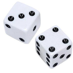$n$ . ⊕
Dice. These dice have six sides each, but we’ll be considering here the more general problem of n-sided dice. We ask, on average, how many times must we throw that die? This problem is at once easier to conceptualize than its continuous counterpart, because it is discrete, and much more difficult to actually calculate—because it is discrete.

Let $K$ be the random variable corresponding to the number of times we must throw the die until the sum of the throws first exceeds $n$ , the number of sides on the die. Ultimately we want to find the probability distribution $P(K=k \mid n)$ — the probability that the sum of our throws first exceeds $n$ after exactly $k$ throws — because once we know this, computing the expected value of $k$ is straightforward via the usual definition:

$\langle k \rangle_n = \sum_{k=2}^{n+1} k P(K=k \mid n)\tag{2}\label{expect}$

Note the limits of summation: we’re running from $2$ to $n+1$ . There is zero chance of exceeding $n$ on the first roll; the best we can do there is $n$ itself. On the other hand, the sum is guaranteed to exceed $n$ after $k = n+1$ rolls, because each roll generates, at minimum, a value of oneNote that although the probability of this sum exceeding n on roll n+1 is unity, that’s not what we’re calculating. We’re calculating the probability that the sum first exceeds n on that roll, and not before, which will be less than one. .

Let $R_i$ represent the random variable corresponding to the $i^{\text{th}}$ roll. The key to calculating $P(K=k \mid n)$ is to realize that it must equal the difference between the following probabilities:

$P(K=k\mid n) = P(K\leq k\mid n) - P(K\leq k-1\mid n) \tag{3}\label{key}$

But note that,

$P(K \leq k \mid n) = P\left(\sum_{i=1}^{k} R_i > n \right) = 1 - P \left( \sum_{i=1}^{k} R_i \leq n \right)\tag{4} \label{complement}$

Using Eq. $\ref{key}$ and Eq. $\ref{complement}$ , we can write $P(K=k \mid n)$ as,

$\begin{align} P(K=k \mid n) &= [1 - P(K \leq k \mid n)] - [1 - P(K \leq k-1 \mid n)] \tag{5}\\ &= P\left(\sum_{i=1}^{k-1} R_i \leq n\right) - P\left(\sum_{i=1}^{k} R_i\leq n\right) \tag{6}\label{prob_diff}\end{align}$

And now we have only to calculate the probability that the sum of $k$ throws is less than or equal to $n$ .

Counting Is Hard

We assume that the $k$ throws are independent events, so the $n^k$ possible outcomes are equally likely. But to compute the probability, we must know, of these outcomes, how many satisfy $\sum_i R_i \leq n$ ? If we call this number $N_{\leq}(n,k)$ , then the probability is,

$P\left(\sum_i R_i \leq n \right) = \frac{N_{\leq}(n, k)}{n^k} \tag{7}\label{prob_div}$

So the problem, then, is to compute $N_{\leq}(n,k)$ for arbitrary $n$ and $k$ .

To find $N_{\leq}$ , let’s first answer a slightly easier question: how many outcomes will sum to exactly $n$ using $k$ integers?

One way to attack this problem is to write out $n$ as the sum of $n$ ones (which sum is guaranteed, of course, to sum to $n$ ), and then consider how many ways we can partition those ones into different groups. This is illustrated in the figure to the right, for the case of $n=6$ and $k=2$ ⊕
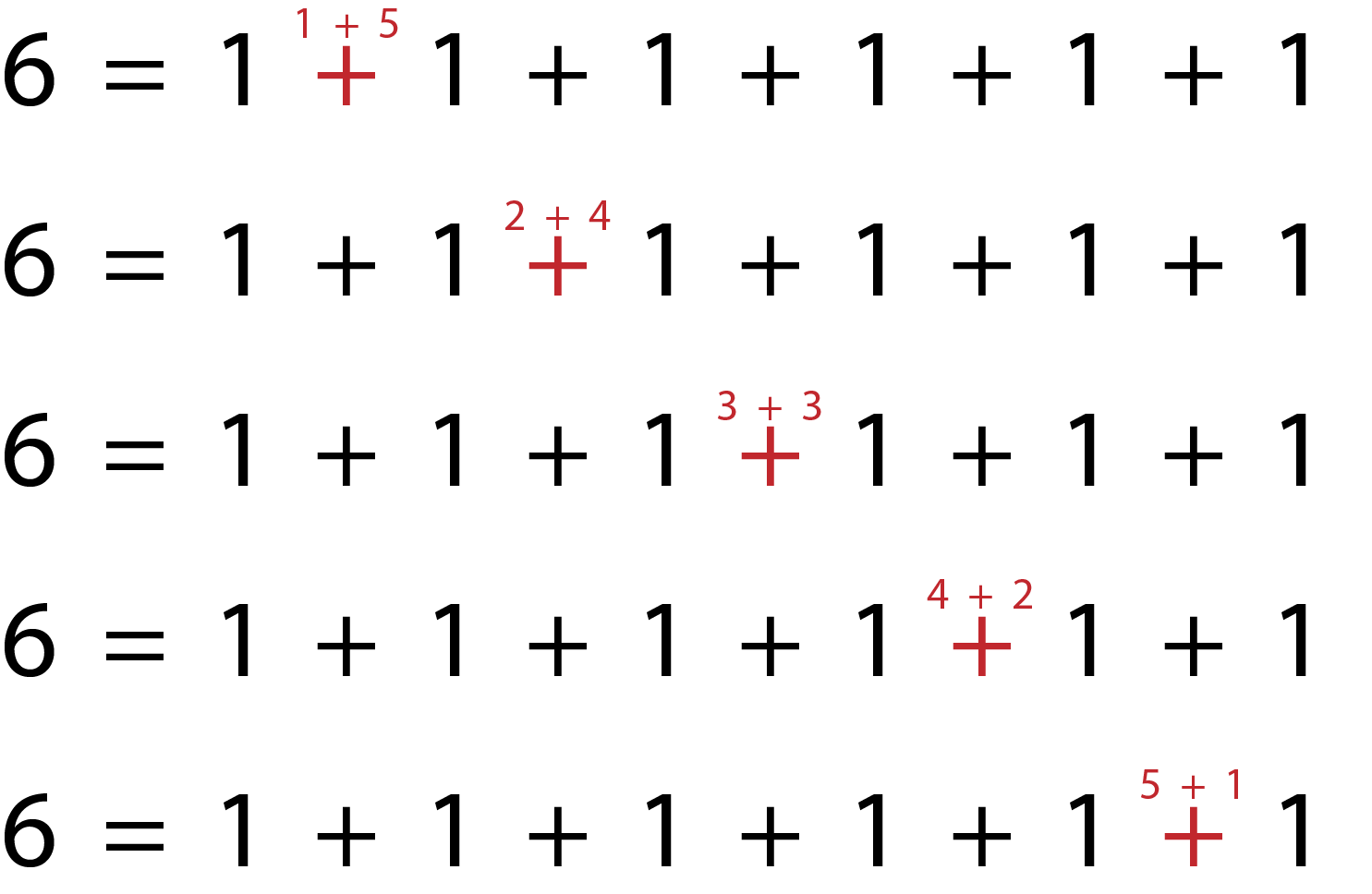
The number of ways we can sum to six via two positive integers is the number of ways we can select one plus sign from among the five plus signs in the equation 6 = 1 + 1 + 1 + 1 + 1 + 1, if we regard the selected plus sign as partitioning the sum into two pieces. The sum to the left of the selected plus sign represents one number, and the sum to the right of that plus sign represents the other. If we wanted to sum to exactly six using three numbers, we’d find the number of ways to select two plus signs from the five available; and so on.. It is easy to see that the partitioning is equivalent to asking, “How many ways can I select one plus sign from the five plus signs?” On the other hand, if we were to ask, how many ways are there to sum to six using three positive integers, we’d want to calculate how many ways we can select two plus signs from those five plus signs, and so forth. This question is answered, in general, using combinations.

Recall that a combination is a selection of items from a collection such that the order of the selection does not matter. The number of ways in which one may select $k$ items from among $n$ available items is given by,

$\binom{n}{k} = \frac{n!}{k!(n - k)!}$

By this argument we see that, in general, the number of ways we can sum to exactly $n$ using $k$ positive integers, which we’ll denote as $N_{=}(n,k)$ , is given by,

$N_{=}(n,k)=\binom{n-1}{k-1}=\frac{(n-1)!}{(k-1)! (n - k + 1)!},$

Using a six-sided die, for example, the number of ways we can sum to six with two throws is given by,

$\binom{6-1}{2-1} = \binom{5}{1} = \frac{5!}{1!4!} = 5$

Note that the five corresponds to the number of possibilities enumerated in the example to the right. This all seems to hang together.

But Eq. $\ref{prob_div}$ requires the total number of outcomes whose sum is less than or equal to $n$ . That number will equal the sum the the number of ways we can reach $n^\prime$ for all $k \leq n^\prime \leq n$ :

$N_{\leq}(n,k) = \sum_{n^\prime=k}^{n} N_=(n^\prime, k) = \sum_{n^\prime=k}^{n} \binom{n^\prime-1}{k-1}=\binom{n}{k}$

where in the last step we’ve used the so-called hockey-stick identity of combinations.

This is a delightfully simple resultDelightful, but hardly surprising. Most interesting counting problems wend their way back to Pascal’s triangle eventually, it seems. that allows us to compute the probability of interest:

$P\left(\sum_{i=1}^{k} R_i \leq n\right) = \frac{1}{n^k} \binom{n}{k} \tag{8} \label{less-than}$

And this, in turn, allows us to calculate the probability in Eq. $\ref{prob_div}$ , $P(K=k \mid n)$ . Using Eq. $\ref{prob_diff}$ and $\ref{less-than}$ ,

$P(K=k) = \frac{1}{n^{k-1}} \binom{n}{k-1} - \frac{1}{n^k} \binom{n}{k} \tag{9} \label{k-is-k}$

And now finally, we’re in a position to compute $\langle k \rangle$ via Eq. $\ref{expect}$ .

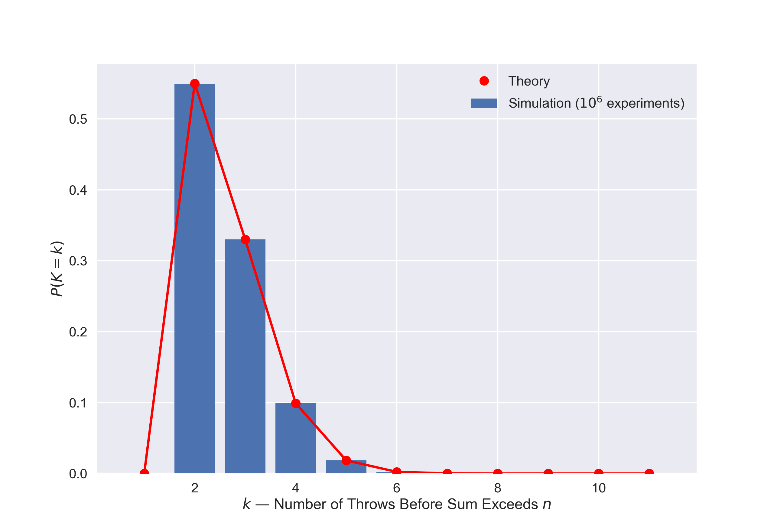
But, well, after all these perambulations, we might wonder if we’ve made a mistake. In these cases, it is prudent to turn to numerical simulation to verify our analytic results. Let’s check our sanity by verifying Eq. $\ref{k-is-k}$ by way of simulation. We do this by simulating our die throwing experiment in Python using a synthetic die with $n=10$ sides, and compare the empirically measured probabilities with our theoretically calculated results, via Eq. $\ref{k-is-k}$ . The results of this, for $10^6$ simulated rounds, is presented in the figure below:

The probability that the sum of successive throws of a ten-sided die exceeds ten, after k throws. Note that the empirical measurements (blue bars) match theoretical predictions (red dots) quite well.

Now that we’ve convinced ourselves that we are correctly computing the probability $P(K=k \mid n)$ , we are finally in a position to calculate the expectation we’re after.

Great Expectations

Before computing $\langle k \rangle$ , let’s rearrange Eq. $\ref{k-is-k}$ to make it a bit simpler. Note that with a little algebra we can write,

$\binom{n}{k-1} = \frac{n!}{(k-1)!(n-k+1)!} = \frac{k}{(n-k+1)}\frac{n!}{k!(n-k)!}=\frac{k}{(n-k+1)}\binom{n}{k}$

This allows us to write Eq. $\ref{k-is-k}$ , with yet a bit more algebra, as,

$P(K=k \mid n) = \frac{n(k-1)+(k-1)}{n^k(n-k+1)} \binom{n}{k}$

Multiplying by $k$ and summing, as per Eq. $\ref{expect}$ , we obtain,

$\langle k \rangle_n = \sum_{k=2}^{n+1}\frac{nk(k-1) + k(k-1)} {n^k(n-k+1)} \binom{n}{k} \tag{10}\label{answer}$

And there we are. For a die with $n$ sides we can now compute the expected number of throws we’ll need to exceed $n$ . What do we expect for a six-sided die? For $n=6$ , Eq. $\ref{answer}$ yields,

$\langle k \rangle_{n=6} = \frac{117649}{46656} \approx 2.522$

a number that is decidedly not $e$ Not that we’d expect it to be, of course; rational numbers tend never to be irrational. . But, interestingly, neither is it too far off. Let’s consider a die with more sides, say, $n=15$ :

$\langle k \rangle_{n=15} = \frac{11152921504606846976}{437893890380859375} \approx 2.633$

Even closer! Intrigued by these observations, let’s keep increasing the number of sides on our die. If we continue calculating the expectation for ever higher values of $n$ , we generate the following plot:

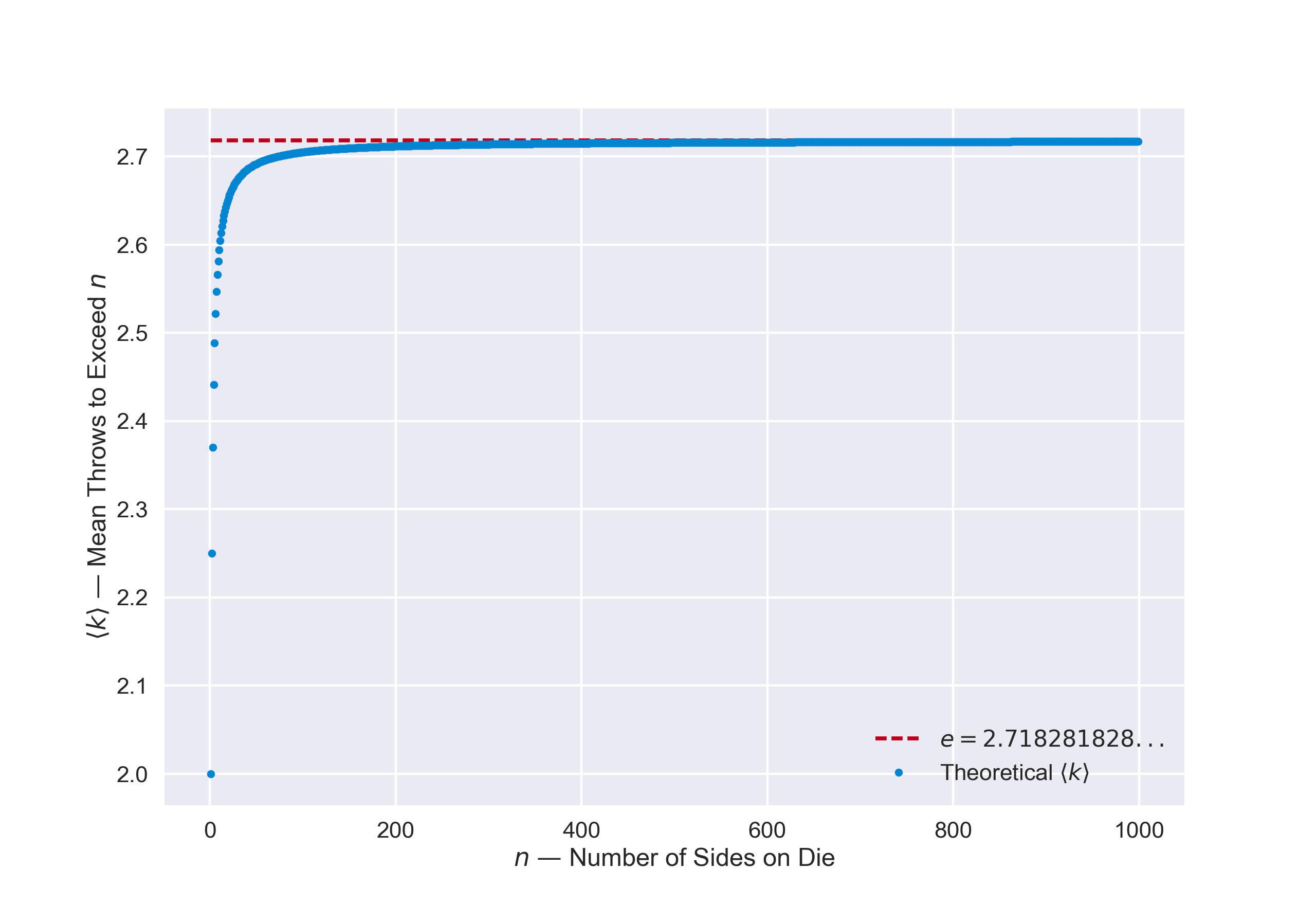
The mean number of die throws required before sum of throws exceeds the number of sides on the die, as a function of the number of sides on the die. Note that this mean value seems to be converging.

It appears that, as we let $n$ increase, the expected number of throws required for the sum to exceed $n$ converges to a number — and that number, empirically at least, appears to be $e$ . But can we prove it? Sure we can.

Let’s write out Eq. $\ref{answer}$ in all its glory,

$\langle k \rangle_n = \sum_{k=2}^{n+1} \frac{n k(k-1) + k(k-1)}{n^k (n-k+1)} \frac{n!}{k!(n-k)!}$

Now consider the case where $n\gg k$ . The above expression simplifies,

$\begin{align} \langle k \rangle_n &\approx \sum_{k=2}^{n+1} \frac{k(k-1)}{n^k}\frac{n!}{k!(n-k)!} \\ &= \sum_{k=2}^{n+1}\frac{n!}{n^k (k-2)! (n-k)!} \\ &= \sum_{k=2}^{n+1}\frac{n! (n-k+2) (n-k+1)}{(k-2)!(n - k + 2)!} \frac{1}{n^k} \\ &\approx \sum_{k=2}^{n} \frac{n!}{(k-2)![n - (k-2)]!} \frac{1}{n^{k-2}} \end{align}$

And now note that we can change the lower limit of the summation; rather than starting at $k=2$ , we can start at $k=0$ , provided we replace all the $(k-2)$ terms that appear in our summand with $k$ . Doing this we obtain,

$\langle k \rangle_n \approx \sum_{k=0}^{n} \frac{1}{n^k} \frac{n!}{k!(n-k)!} = \sum_{k=0}^{n} \frac{1}{n^k} \binom{n}{k}$

where, again, this holds for $n \gg k$ . This may begin to look familiar. In particular, recall the binomial theorem, which states that,

$(1+x)^n = \sum_{k=0}^n x^k \binom{n}{k}$

In our present situation, letting $x = 1/n$ , we can write our expectation as,

$\lim_{n \rightarrow \infty} \langle k \rangle_n = \lim_{n \rightarrow \infty} \sum_{k=0}^{n} \frac{1}{n^k} \binom{n}{k} = \lim_{n \rightarrow \infty} \left(1+ \frac{1}{n}\right)^n \equiv e$

And we’ve recovered the definition of Euler’s number, à la Eq. $\ref{edef}$ !

Here is where I find $e$ emerge organically, in a sense. For all finite values of $n$ , the expectation is a rational number. But as the number of sides increases, the combinatorics of how the throws can sum to exceed $n$ evolves in just the right way such that—as $n$ gets really large—it starts to converge to the binomial expansion of $(1+1/n)^n$ , which in the limit turns out to be exactly the definition of $e$ . And for my part, at least, I can start to see a glimmer of an answer to that primal question: who ordered that?Of course, you might argue, the other proofs I’ve cited could be brought to this same point—the binomial expansion could ultimately be reconstructed from those calculations as well. Certainly, I’d agree, they must all be equivalent at some level, but seeing the binomial theorem emerge directly from the combinatorics of die throws and lead to the very definition of Euler’s constant makes me feel happy inside.

From Discrete Back to Continuous

As $n$ heads off to infinity, our discrete problem becomes equivalent to the original, continuous problem introduced at the start. To better see the equivalence, note we can map the discrete problem onto the unit interval, as in the following illustration.

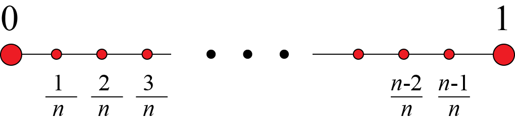
We can reconstruct our discrete die-throwing experiment on the unit interval by partitioning it into subintervals. As the number of subintervals approaches infinity—equivalent to our infinite sided die—we recover the uniform distribution we introduced about originally.

Rather than considering an $n$ -sided die, we partition the unit interval into $n$ subintervals. At each step, we then sample a number uniformly from the interval $[0,1]$ , and select as our value the uppermost limit of whatever subinterval the sample falls into. We continue to select values in this manner until their sum exceeds one, just as in the original formulation of the problem—but now we’re working in the context of a discrete problem. And now, as $n \rightarrow \infty$ , discrete meets continuous, and by the arguments advanced above, we’ve proven the original assertion.